Synthetic Data#
The specreduce.utils.synth_data module provides SynthImage,
a composable builder for generating synthetic 2D spectroscopic images. It is primarily used to
create test data and documentation examples, but is also a convenient way to explore how the
reduction tools respond to known inputs.
The builder#
SynthImage is immutable and chainable. You start from an
empty canvas of a given size, add signal layers and noise, and finally render the result with
one of the to_* methods. Each add_* call returns a new SynthImage, so the original is
never modified and a base configuration can be branched safely:
base = SynthImage(nx=1024, ny=512).add_background(5)
arc = base.add_arcs(["HeI"])        # base is unchanged
spec = base.add_source()            # an independent branch
Signal layers are additive and stackable:
add_background()adds a constant level.add_source()adds a source whose spatial profile follows a Chebyshev trace (call it more than once for multiple sources). By default the source is a flat continuum, but passing a 1DSpectrummodulates the flux along the dispersion axis: the spectrum is resampled onto the image wavelength grid, normalized to a peak of one, and zeroed outside its wavelength range.add_arcs()adds emission lines from one or morepypeitcalibration line lists, with an optional cross-dispersion tilt.add_skylines()is a convenience wrapper aroundadd_arcsfor night-sky airglow (OH) line lists.
Noise is applied last, regardless of the order in which it is added, in physical order (Poisson, then read noise):
add_poisson_noise()applies photon (Poisson) noise.add_read_noise()(aliasadd_rdnoise()) adds Gaussian read noise.
Both noise stages draw from a single generator seeded by the seed argument, so a seeded
SynthImage renders reproducibly; with seed=None the noise is non-deterministic.
Finally, render the image with
to_array() (a ndarray),
to_ccddata() (a CCDData), or
to_spectrum() (a Spectrum).
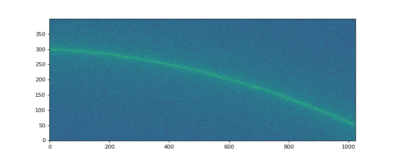
The following example builds a traced continuum source with a constant background, Poisson noise,
and read noise, then renders it to a CCDData:
import matplotlib.pyplot as plt
from astropy.modeling import models
from specreduce.utils.synth_data import SynthImage

image = (
    SynthImage(nx=1024, ny=400, seed=42)
    .add_background(5)
    .add_source(profile=models.Moffat1D(amplitude=20, alpha=0.1))
    .add_poisson_noise()
    .add_read_noise(3)
    .to_ccddata()
)
plt.figure(figsize=(10, 4))
plt.imshow(image, origin="lower", aspect="auto")
(Source code, png, hires.png, pdf)

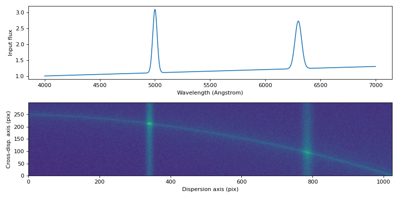
A source with a wavelength-dependent spectrum#
By default a source is a flat continuum, but passing a 1D Spectrum to
add_source() modulates its flux along the dispersion
axis. The spectrum is resampled onto the image wavelength grid, normalized to a peak of one, and
zeroed outside its wavelength range. The example below builds a continuum with two emission lines and
renders a traced source whose brightness follows it (no network access required):
import matplotlib.pyplot as plt
import numpy as np
import astropy.units as u
from astropy.modeling import models
from specutils import Spectrum
from specreduce.utils.synth_data import SynthImage

# a rising continuum with two emission lines
wave = np.linspace(4000, 7000, 1000) * u.Angstrom
continuum = 1.0 + 0.3 * (wave.value - 4000) / 3000
emission = (
    2.0 * np.exp(-0.5 * ((wave.value - 5000) / 20) ** 2)
    + 1.5 * np.exp(-0.5 * ((wave.value - 6300) / 30) ** 2)
)
spectrum = Spectrum(flux=(continuum + emission) * u.count, spectral_axis=wave)

image = (
    SynthImage(nx=1024, ny=300, extent=(4000, 7000), seed=42)
    .add_background(5)
    .add_source(profile=models.Moffat1D(amplitude=50, alpha=0.1), spectrum=spectrum)
    .add_poisson_noise()
    .to_ccddata()
)

fig, (ax1, ax2) = plt.subplots(2, 1, figsize=(10, 5))
ax1.plot(wave, spectrum.flux)
ax1.set_xlabel("Wavelength (Angstrom)")
ax1.set_ylabel("Input flux")
ax2.imshow(image, origin="lower", aspect="auto")
ax2.set_xlabel("Dispersion axis (pix)")
ax2.set_ylabel("Cross-disp. axis (pix)")
fig.tight_layout()
(Source code, png, hires.png, pdf)

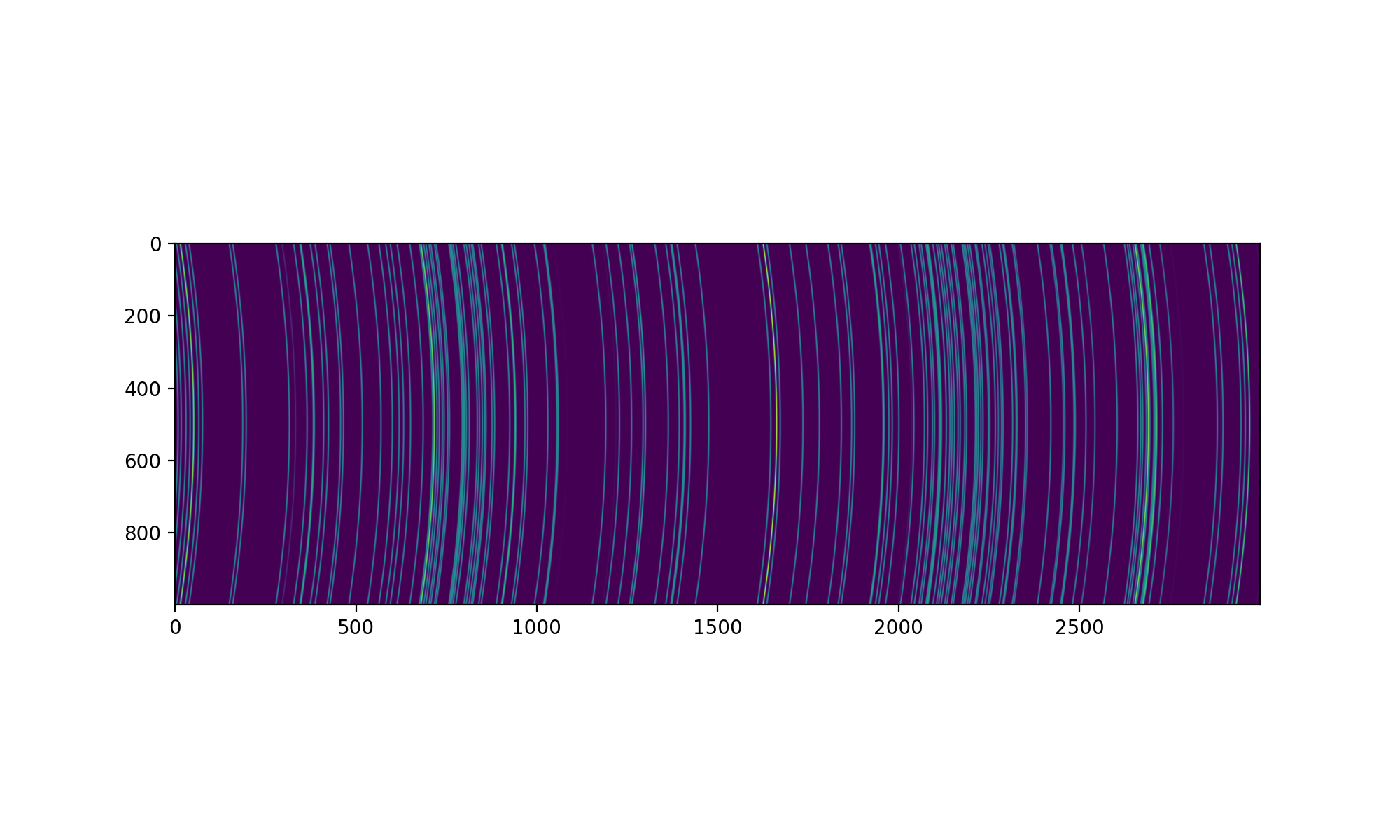
Tilted and curved arc lines#
This is an example of modeling a spectrograph whose output is curved in the cross-dispersion direction:
import matplotlib.pyplot as plt
import numpy as np
from astropy.modeling import models
import astropy.units as u
from specreduce.utils.synth_data import SynthImage

model_deg2 = models.Legendre1D(degree=2, c0=50, c1=0, c2=100)
im = (
    SynthImage(nx=3000, ny=1000)
    .add_background(5)
    .add_arcs(['HeI', 'ArI', 'ArII'], line_fwhm=3, tilt_func=model_deg2)
    .add_poisson_noise()
    .to_ccddata()
)
fig = plt.figure(figsize=(10, 6))
plt.imshow(im)
(Source code, png, hires.png, pdf)
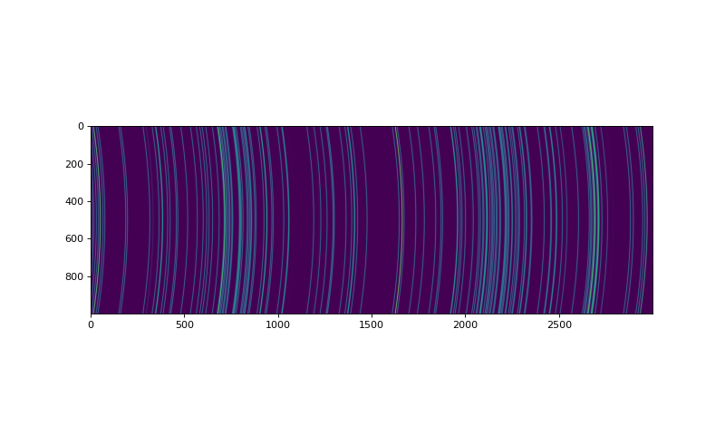
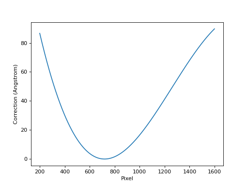
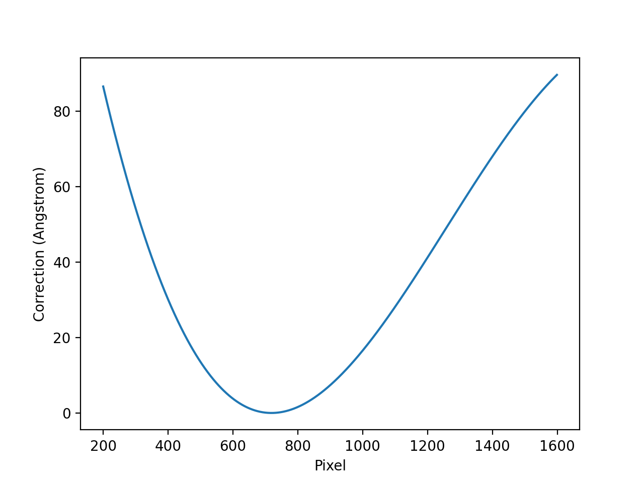
Modeling a non-linear dispersion relation#
The FITS WCS standard implements ideal world coordinate functions based on the physics
of simple dispersers. This is described in detail by Paper III,
https://www.aanda.org/articles/aa/pdf/2006/05/aa3818-05.pdf. This can be used to model a
non-linear dispersion relation based on the properties of a spectrograph. This example
recreates Figure 5 in that paper using a spectrograph with a 450 lines/mm volume phase
holographic grism. Standard gratings only use the first three PV terms:
import numpy as np
import matplotlib.pyplot as plt
from astropy.wcs import WCS
import astropy.units as u
from specreduce.utils.synth_data import SynthImage

non_linear_header = {
    'CTYPE1': 'AWAV-GRA',  # Grating dispersion function with air wavelengths
    'CUNIT1': 'Angstrom',  # Dispersion units
    'CRPIX1': 719.8,       # Reference pixel [pix]
    'CRVAL1': 7245.2,      # Reference value [Angstrom]
    'CDELT1': 2.956,       # Linear dispersion [Angstrom/pix]
    'PV1_0': 4.5e5,        # Grating density [1/m]
    'PV1_1': 1,            # Diffraction order
    'PV1_2': 27.0,         # Incident angle [deg]
    'PV1_3': 1.765,        # Reference refraction
    'PV1_4': -1.077e6,     # Refraction derivative [1/m]
    'CTYPE2': 'PIXEL',     # Spatial detector coordinates
    'CUNIT2': 'pix',       # Spatial units
    'CRPIX2': 1,           # Reference pixel
    'CRVAL2': 0,           # Reference value
    'CDELT2': 1            # Spatial units per pixel
}

linear_header = {
    'CTYPE1': 'AWAV',  # Grating dispersion function with air wavelengths
    'CUNIT1': 'Angstrom',  # Dispersion units
    'CRPIX1': 719.8,       # Reference pixel [pix]
    'CRVAL1': 7245.2,      # Reference value [Angstrom]
    'CDELT1': 2.956,       # Linear dispersion [Angstrom/pix]
    'CTYPE2': 'PIXEL',     # Spatial detector coordinates
    'CUNIT2': 'pix',       # Spatial units
    'CRPIX2': 1,           # Reference pixel
    'CRVAL2': 0,           # Reference value
    'CDELT2': 1            # Spatial units per pixel
}

non_linear_wcs = WCS(non_linear_header)
linear_wcs = WCS(linear_header)

# this re-creates Paper III, Figure 5
pix_array = 200 + np.arange(1400)
nlin = non_linear_wcs.spectral.pixel_to_world(pix_array)
lin = linear_wcs.spectral.pixel_to_world(pix_array)
resid = (nlin - lin).to(u.Angstrom)
plt.plot(pix_array, resid)
plt.xlabel("Pixel")
plt.ylabel("Correction (Angstrom)")
plt.show()
(Source code, png, hires.png, pdf)

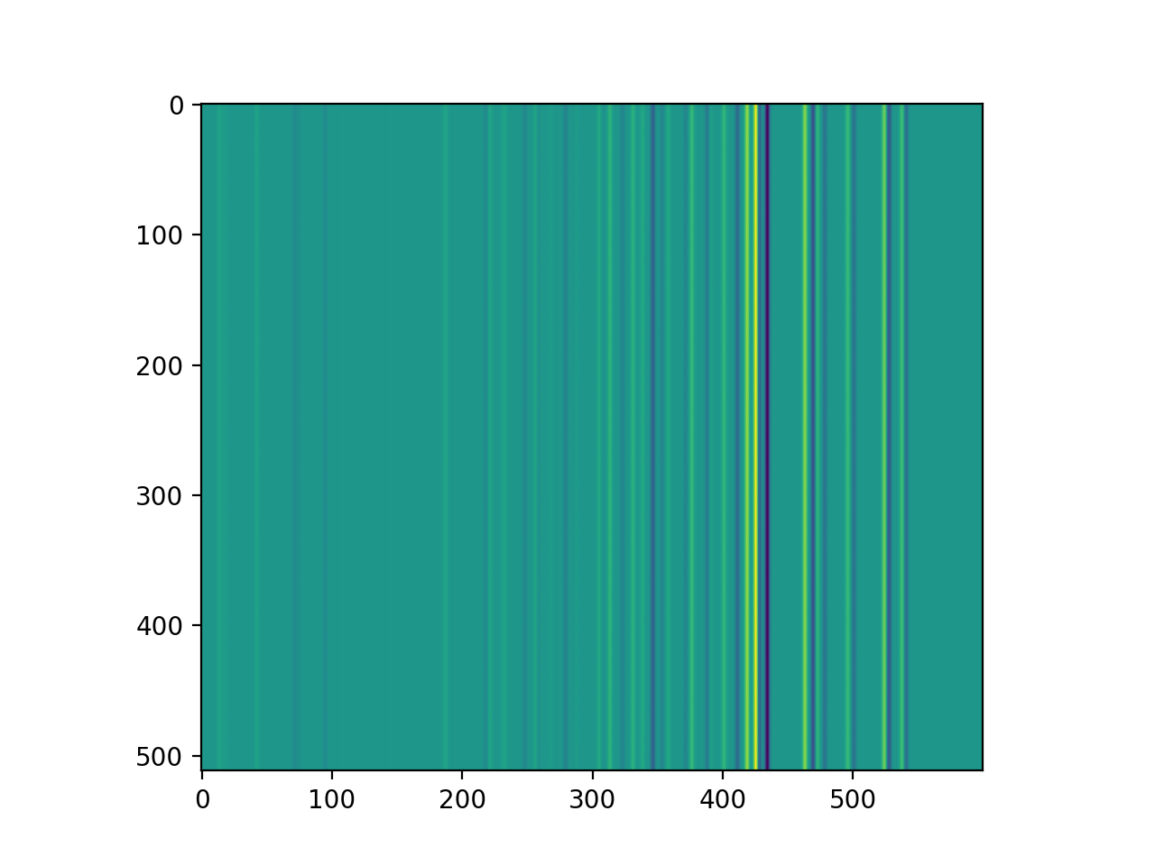
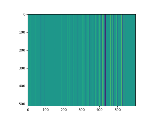
nlin_im = (
    SynthImage(nx=600, ny=512, wcs=non_linear_wcs)
    .add_background(5)
    .add_arcs(['HeI', 'NeI'], line_fwhm=3, wave_air=True)
    .add_poisson_noise()
    .to_ccddata()
)
lin_im = (
    SynthImage(nx=600, ny=512, wcs=linear_wcs)
    .add_background(5)
    .add_arcs(['HeI', 'NeI'], line_fwhm=3, wave_air=True)
    .add_poisson_noise()
    .to_ccddata()
)

# subtracting the linear simulation from the non-linear one shows how the
# positions of lines diverge between the two cases
plt.imshow(nlin_im.data - lin_im.data)
plt.show()
Note
The older make_2d_trace_image, make_2d_arc_image, and make_2d_spec_image
functions are deprecated in favor of SynthImage and will be
removed in a future release.