Spectrophotometric Standards#
Introduction#
Instrument sensitivity as a function of wavelength is calibrated using observations of
spectrophotometric standard stars. specreduce offers some
convenience functions for accessing some databases of commonly used standard stars and loading the data into Spectrum
instances.
Supported Databases#
Probably the most well-curated database of spectrophotometric calibration data is the
CALSPEC
database at MAST (Ref.: Bohlin, Gordon, & Tremblay 2014).
It also has the advantage of including data that extends well into both the UV and the IR. The load_MAST_calspec
function provides a way to easily load CALSPEC data either directly from MAST
(specifically, https://archive.stsci.edu/hlsps/reference-atlases/cdbs/calspec/) or from a previously downloaded local file.
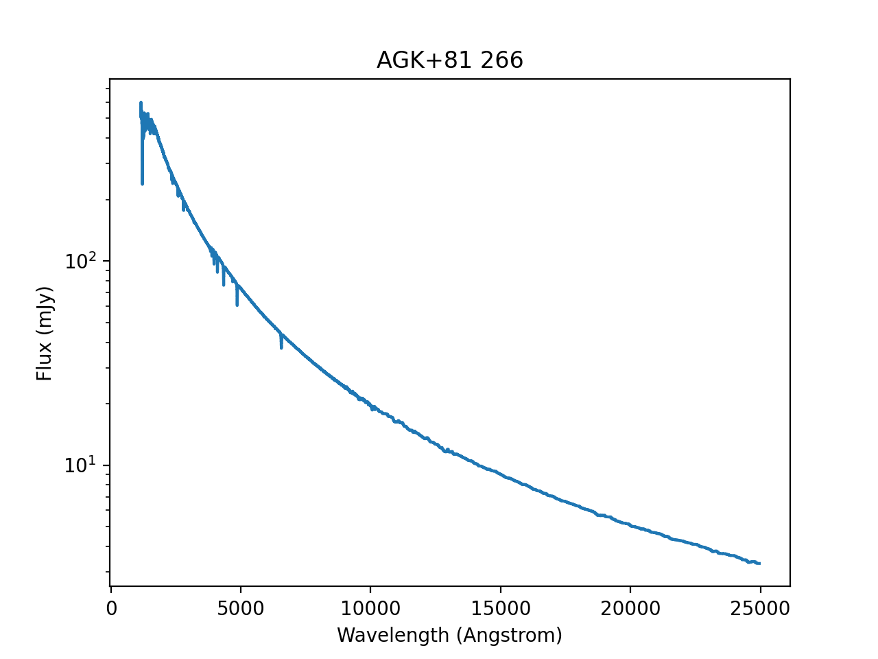
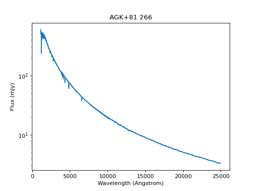
Here is an example of how to use it and of a CALSPEC standard that has both UV and IR coverage:
import matplotlib.pyplot as plt
from specreduce.calibration_data import load_MAST_calspec

spec = load_MAST_calspec("agk_81d266_stisnic_007.fits")

fig, ax = plt.subplots()
ax.step(spec.spectral_axis, spec.flux, where="mid")
ax.set_yscale('log')
ax.set_xlabel(f"Wavelength ({spec.spectral_axis.unit})")
ax.set_ylabel(f"Flux ({spec.flux.unit})")
ax.set_title("AGK+81 266")
fig.show()
(Source code, png, hires.png, pdf)
The specreduce_data package provides several datasets of spectrophotometric standard spectra.
The bulk of them are inherited from IRAF’s onedstds datasets, but
some more recently curated datasets from ESO, the
Nearby Supernova Factory, and Gemini are included as well. The
load_onedstds function is provided to load these data into Spectrum
instances. If specreduce_data is not installed, the data will be downloaded from the GitHub
repository. The available
database names and their descriptions are listed here. Please refer to the specreduce-data repository for details on the
specific data files that are available:
bstdscal: Directory of the brighter KPNO IRS standards (i.e., those with HR numbers) at 29 bandpasses, data from various sources transformed to the Hayes and Latham system, unpublished.
ctiocal: Directory containing fluxes for the southern tertiary standards as published by Baldwin & Stone, 1984, MNRAS, 206, 241 and Stone and Baldwin, 1983, MNRAS, 204, 347.
ctionewcal: Directory containing fluxes at 50 Å steps in the blue range 3300-7550 Å for the tertiary standards of Baldwin and Stone derived from the revised calibration of Hamuy et al., 1992, PASP, 104, 533. This directory also contains the fluxes of the tertiaries in the red (6050-10000 Å) at 50 Å steps as will be published in PASP (Hamuy et al 1994). The combined fluxes are obtained by gray shifting the blue fluxes to match the red fluxes in the overlap region of 6500-7500 Å and averaging the red and blue fluxes in the overlap. The separate red and blue fluxes may be selected by following the star name with “red” or “blue”; i.e. CD 32 blue.
iidscal: Directory of the KPNO IIDS standards at 29 bandpasses, data from various sources transformed to the Hayes and Latham system, unpublished.
irscal: Directory of the KPNO IRS standards at 78 bandpasses, data from various sources transformed to the Hayes and Latham system, unpublished (note that in this directory the brighter standards have no values - the bstdscal directory must be used for these standards).
oke1990: Directory of spectrophotometric standards observed for use with the HST, Table VII, Oke 1990, AJ, 99, 1621 (no correction was applied). An arbitrary 1 Å bandpass is specified for these smoothed and interpolated flux “points”.
redcal: Directory of standard stars with flux data beyond 8370 Å. These stars are from the IRS or the IIDS directory but have data extending as far out into the red as the literature permits. Data from various sources.
spechayescal: The KPNO spectrophotometric standards at the Hayes flux points, Table IV, Spectrophotometric Standards, Massey et al., 1988, ApJ 328, p. 315.
spec16cal: Directory containing fluxes at 16 Å steps in the blue range 3300-7550 Å for the secondary standards, published in Hamuy et al., 1992, PASP, 104, 533. This directory also contains the fluxes of the secondaries in the red (6020-10300 Å) at 16 Å steps as will be published in PASP (Hamuy et al 1994). The combined fluxes are obtained by gray shifting the blue fluxes to match the red fluxes in the overlap region of 6500-7500 Å and averaging the blue and red fluxes in the overlap. The separate red and blue fluxes may be selected by following the star name with “red” or “blue”; i.e. HR 1544 blue.
spec50cal: The KPNO spectrophotometric standards at 50 Å intervals. The data are from (1) Table V, Spectrophotometric Standards, Massey et al., 1988, ApJ 328, p. 315 and (2) Table 3, The Kitt Peak Spectrophotometric Standards: Extension to 1 micron, Massey and Gronwall, 1990, ApJ 358, p. 344.
snfactory: Preferred standard stars from the LBL Nearby Supernova Factory project: https://ui.adsabs.harvard.edu/abs/2002SPIE.4836…61A/abstract Data compiled from https://snfactory.lbl.gov/snf/snf-specstars.html. See notes there for details and references.
eso: Directories of spectrophotometric standards copied from ftp://ftp.eso.org/pub/stecf/standards/. See https://www.eso.org/sci/observing/tools/standards/spectra/stanlis.html for links, notes, and details.
gemini: Directory of spectrophotometric standards used by Gemini. Originally copied from GeminiDRSoftware/DRAGONS.
Selecting Spectrophotometric Standard Stars#
Many commonly used standard stars have spectra in multiple datasets, but the quality and systematics can differ.
The load_MAST_calspec and load_onedstds functions can be
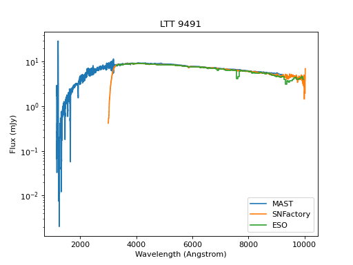
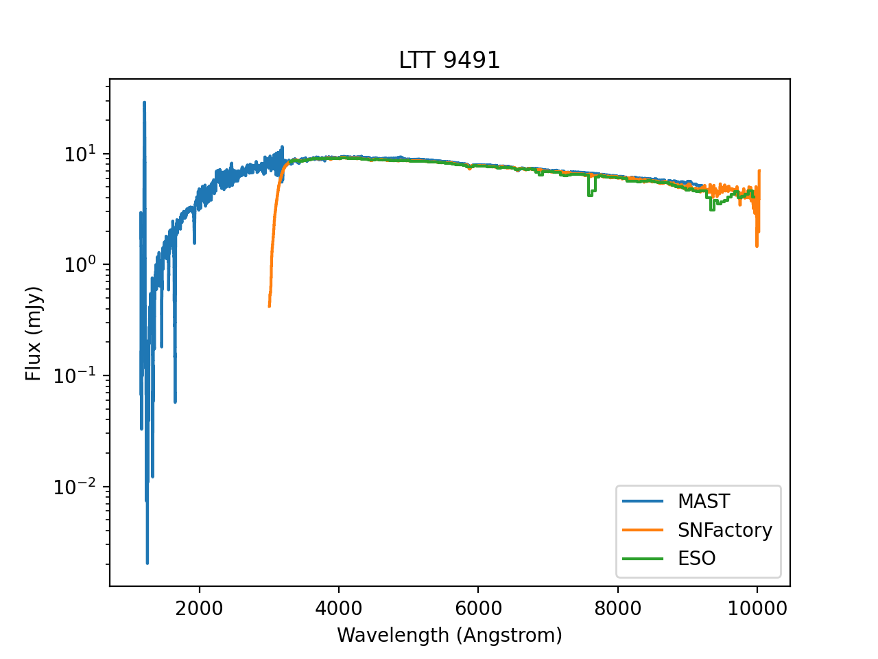
useful tools for exploring and comparing spectra from the various databases. An example is shown here for LTT 9491 which has
spectra available from MAST, ESO, and the Nearby Supernova factory:
import matplotlib.pyplot as plt
from specreduce.calibration_data import load_MAST_calspec, load_onedstds

s1 = load_MAST_calspec("ltt9491_002.fits")
s2 = load_onedstds("snfactory", "LTT9491.dat")
s3 = load_onedstds("eso", "ctiostan/ltt9491.dat")

fig, ax = plt.subplots()
ax.step(s1.spectral_axis, s1.flux, label="MAST", where="mid")
ax.step(s2.spectral_axis, s2.flux, label="SNFactory", where="mid")
ax.step(s3.spectral_axis, s3.flux, label="ESO", where="mid")
ax.set_yscale('log')
ax.set_xlabel(f"Wavelength ({s1.spectral_axis.unit})")
ax.set_ylabel(f"Flux ({s1.flux.unit})")
ax.set_title("LTT 9491")
ax.legend()
fig.show()
(Source code, png, hires.png, pdf)

The MAST data have the best UV coverage, but that’s not useful from the ground and they only extend to 0.9 microns in the red in this case. The other data extend to 1.0 microns, but both spectra show systematics due to telluric absorption. The SNFactory data extend well past the atmospheric cutoff with no correction applied for atmospheric transmission. The ESO data, on the other hand, are not corrected for the telluric features in the near-IR while the SNFactory data are. Regions affected by such telluric systematics should be masked out before these spectra are used for calibration purposes.