Atmospheric Extinction#
Introduction#
The Earth’s atmosphere is highly chromatic in its transmission of light. The wavelength-dependence is dominated by scattering in the optical (320-700 nm) and molecular features in the near-infrared and infrared.
Supported Optical Extinction Models#
specreduce offers support for average optical extinction models for a set of observatories:
Model Name |
Observatory |
Lat |
Lon |
Elevation (m) |
Ref |
|---|---|---|---|---|---|
ctio |
Cerro Tololo Int’l Observatory |
-30.165 |
70.815 |
2215 |
1 |
kpno |
Kitt Peak Nat’l Observatory |
31.963 |
111.6 |
2120 |
2 |
lapalma |
Roque de Los Muchachos Observatory |
28.764 |
17.895 |
2396 |
3 |
mko |
Mauna Kea Int’l Observatory |
19.828 |
155.48 |
4160 |
4 |
mtham |
Lick Observatory, Mt. Hamilton Station |
37.341 |
121.643 |
1290 |
5 |
paranal |
European Southern Obs., Paranal Station |
-24.627 |
70.405 |
2635 |
6 |
apo |
Apache Point Observatory |
32.780 |
105.82 |
2788 |
7 |
1. The CTIO extinction curve was originally distributed with IRAF and comes from the work of Stone & Baldwin (1983 MN 204, 347) plus Baldwin & Stone (1984 MN 206, 241). The first of these papers lists the points from 3200-8370A while the second extended the flux calibration from 6056 to 10870A but the derived extinction curve was not given in the paper. The IRAF table follows SB83 out to 6436, the redder points presumably come from BS84 with averages used in the overlap region. More recent CTIO extinction curves are shown as Figures in Hamuy et al (92, PASP 104, 533 ; 94 PASP 106, 566).
2. The KPNO extinction table was originally distributed with IRAF. The ultimate provenance of this data is unclear, but it has been used as-is in this form for over 30 years.
3. Extinction table for Roque de Los Muchachos Observatory, La Palma. Described in https://www.ing.iac.es/Astronomy/observing/manuals/ps/tech_notes/tn031.pdf.
4. Median atmospheric extinction data for Mauna Kea Observatory measured by the Nearby SuperNova Factory: https://www.aanda.org/articles/aa/pdf/2013/01/aa19834-12.pdf.
5. Extinction table for Lick Observatory on Mt. Hamilton constructed from https://mthamilton.ucolick.org/techdocs/standards/lick_mean_extinct.html.
6. Updated extinction table for ESO-Paranal taken from https://www.aanda.org/articles/aa/pdf/2011/03/aa15537-10.pdf.
7. Extinction table for Apache Point Observatory. Based on the extinction table used for SDSS and available at https://www.apo.nmsu.edu/arc35m/Instruments/DIS/ (https://www.apo.nmsu.edu/arc35m/Instruments/DIS/images/apoextinct.dat).
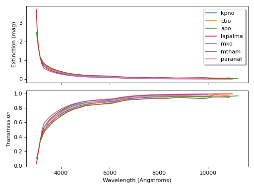
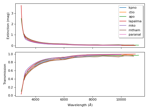
In each case, the extinction is given in magnitudes per airmass and the wavelengths are in Angstroms. Here is an example that
uses the AtmosphericExtinction class to load each model and plots the extinction in magnitudes as well
as fractional transmission as a function of wavelength:
import matplotlib.pyplot as plt
from specreduce.calibration_data import AtmosphericExtinction, SUPPORTED_EXTINCTION_MODELS

fig, ax = plt.subplots(2, 1, sharex=True)
for model in SUPPORTED_EXTINCTION_MODELS:
    ext = AtmosphericExtinction(model=model)
    ax[0].plot(ext.spectral_axis, ext.extinction_mag, label=model)
    ax[1].plot(ext.spectral_axis, ext.transmission)
ax[0].legend(fancybox=True, shadow=True)
ax[1].set_xlabel("Wavelength (Angstroms)")
ax[0].set_ylabel("Extinction (mag)")
ax[1].set_ylabel("Transmission")
plt.tight_layout()
fig.show()
(Source code, png, hires.png, pdf)
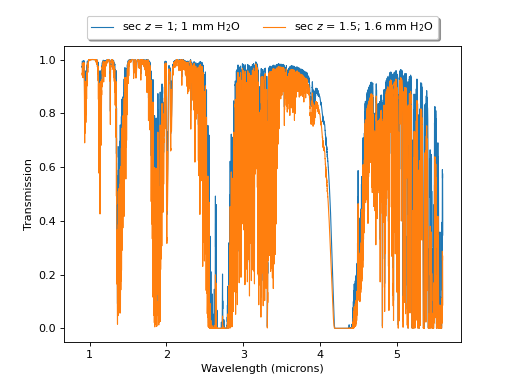
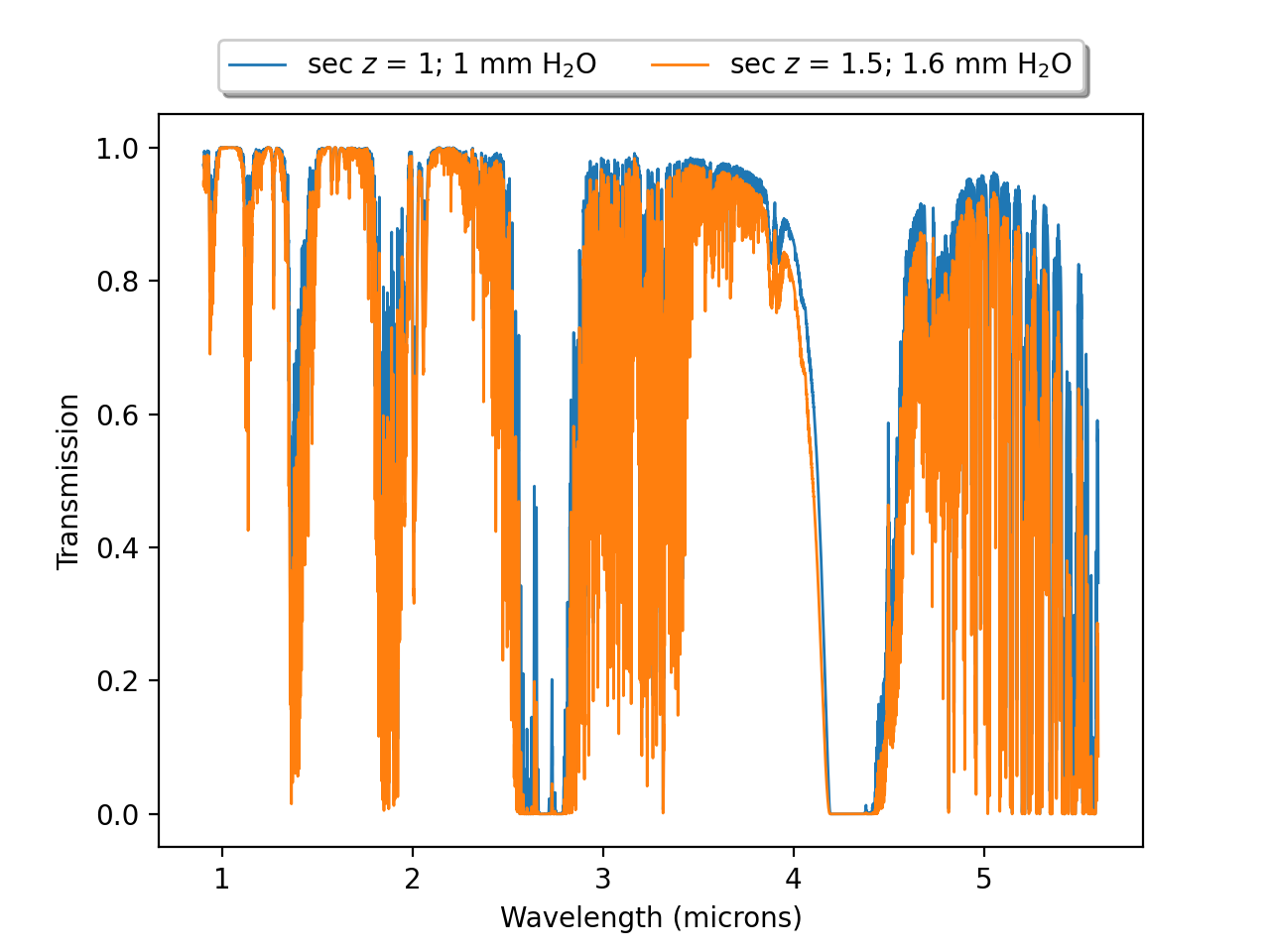
A convenience class, AtmosphericTransmission, is provided for loading data files containing atmospheric transmission
versus wavelength. The common use case for this would be loading the output of telluric models. By default it loads a telluric model for an
airmass of 1 and 1 mm of precipitable water. Some resources for generating more realistic model atmospheric transmission spectra include
https://mwvgroup.github.io/pwv_kpno/1.0.0/documentation/html/index.html and http://www.eso.org/sci/software/pipelines/skytools/molecfit.
import matplotlib.pyplot as plt
from specreduce.calibration_data import AtmosphericTransmission, SUPPORTED_EXTINCTION_MODELS

fig, ax = plt.subplots()
ext_default = AtmosphericTransmission()
ext_custom = AtmosphericTransmission(data_file="atm_transmission_secz1.5_1.6mm.dat")
ax.plot(ext_default.spectral_axis, ext_default.transmission, label=r"sec $z$ = 1; 1 mm H$_{2}$O", linewidth=1)
ax.plot(ext_custom.spectral_axis, ext_custom.transmission, label=r"sec $z$ = 1.5; 1.6 mm H$_{2}$O", linewidth=1)
ax.legend(loc="upper center", bbox_to_anchor=(0.5, 1.12), ncol=2, fancybox=True, shadow=True)
ax.set_xlabel("Wavelength (microns)")
ax.set_ylabel("Transmission")
fig.show()
(Source code, png, hires.png, pdf)
