2D Tilt Correction#

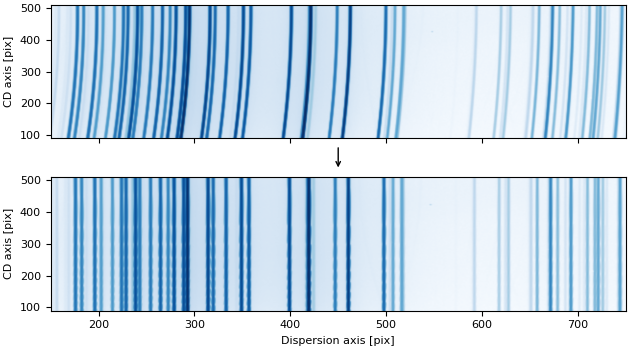
Tilt correction is a calibration step that addresses optical distortions and misalignments in spectroscopic instruments. These distortions cause wavelength to vary along the cross-dispersion (spatial) axis, resulting in spectral features appearing tilted or curved across the detector rather than being perfectly aligned with detector columns.

Tilt correction is performed by modeling a two-dimensional tilt function that describes how wavelength positions shift across the spatial axis. This function can be determined empirically from arc lamp calibration spectra by measuring how the centroids of emission lines vary along the cross-dispersion axis.

Once characterized, the tilt function enables transformation of two-dimensional spectroscopic images so that wavelengths become aligned along straight lines parallel to the detector axes. This alignment is important for achieving accurate wavelength calibration and performing robust sky subtraction.

The specreduce library provides two complementary classes for 2D tilt correction:

TiltCorrection: a high-level calibration workflow to detect arc lines across the detector, fit a 2D polynomial tilt model, and inspect the results.
TiltSolution: a lightweight solution container that holds the tilt-corrected-to-detector coordinate transform and provides flux-conserving 2D resampling.

The tilt function is represented as a 2D polynomial using an Polynomial2D instance. A typical workflow involves:

Initialization: Create an instance with arc lamp data, a trace, or a reference pixel position.
Line Detection: Identify emission lines across the detector.
Fitting: Fit a 2D polynomial model to characterize the geometric distortion.
Inspection: Assess fit quality using diagnostic plots.
Applying the Solution: Use the fitted solution to tilt-correct observed frames.

Quickstart#

1. Initialization#

You instantiate TiltCorrection by providing one or more arc lamp calibration frames and a Trace object. The trace automatically sets the reference positions used to center the tilt model:

from specreduce.tilt_correction import TiltCorrection

tc = TiltCorrection(arc_frames=arc, trace=trace)

Alternatively, you can specify the reference positions manually without a trace:

tc = TiltCorrection(arc_frames=arc, cdisp_ref_pixel=512)

Key parameters:

arc_frames: One or more arc lamp frames as NDData instances (or a sequence of them). Multiple arc frames are supported for combining different lamps.
trace: A Trace object representing the spectrum trace. When provided, the reference pixel is derived automatically.
cdisp_ref_pixel: The reference pixel position along the cross-dispersion axis. Should be close to the trace’s average cross-dispersion position for best results. Determined automatically if a trace is provided.
disp_ref_pixel: The reference pixel position along the dispersion axis. Defaults to the center of the frame if not provided. Determined automatically if a trace is provided.
n_cdisp_samples: Number of cross-dispersion sample positions to generate (default 10). Arc lines are measured at each sample position to characterize how line centroids shift across the spatial axis.
cdisp_sample_lims: Tuple (min, max) specifying the range for cross-dispersion sampling. Defaults to the full extent of the frame.
cdisp_samples: An explicit list of cross-dispersion positions to use instead of automatically generated ones. Overrides n_cdisp_samples if provided.
mask_treatment: Controls how masked or non-finite values are handled in the input image. Accepts any of the standard specreduce masking options ("apply", "ignore", "propagate", "zero_fill", "nan_fill", "apply_mask_only", "apply_nan_only").

2. Finding Arc Lines#

After initialization, detect emission lines at the reference row and at each cross-dispersion sample position using find_arc_lines():

tc.find_arc_lines(fwhm=3.5, noise_factor=5)

This method:

Identifies line centroids at the reference row (set by cdisp_ref_pixel) — these define the “ideal” line positions.
Identifies line centroids at each cross-dispersion sample position.
Builds KD-trees from the sample positions for efficient nearest-neighbor matching during the fitting step.

Parameters:

fwhm: Expected full width at half maximum of the spectral lines (in pixels), used by the line-finding algorithm.
noise_factor: Multiplier for noise thresholding — lines below noise_factor × noise_level are rejected. Default is 5.

3. Fitting the Tilt Model#

Fit a 2D polynomial model that maps coordinates from the tilt-corrected space to detector space using fit():

tc.fit(degree=4, max_distance=10)

The fitting proceeds in two stages:

Initial optimization: Uses scipy.optimize.minimize to minimize the sum of distances between the transformed sample positions and their nearest neighbors in detector space (via the KD-trees).
Least-squares refinement: Automatically calls refine_fit() to perform a least-squares fit on matched line pairs, using the initial solution as the starting point.

Parameters:

degree: Degree of the final Polynomial2D model.
method: Optimization method for the initial stage (default "Powell").
max_distance: Maximum distance for nearest-neighbor matching during the initial fit.

After the initial fit, you can further refine the solution with tighter matching constraints:

tc.refine_fit(degree=4, match_distance_bound=3.0)

This is useful for iteratively tightening the match distance to reject outliers and improve the polynomial fit.

4. Inspecting the Fit#

Several diagnostic tools help assess the quality of the tilt solution:

Residual visualization: Use plot_fit_quality() to see a 2D scatter of matched lines with 1D residual projections along both axes:
```
fig = tc.plot_fit_quality(max_match_distance=5)
```
Wavelength contours: Use plot_wavelength_contours() to overlay constant-wavelength contour lines on a detector image, verifying that the tilt model aligns with the arc features:
```
import matplotlib.pyplot as plt

fig, ax = plt.subplots()
ax.imshow(arc.data, origin="lower", aspect="auto")
tc.plot_wavelength_contours(ax=ax, n_disp=50)
```

5. Using the Tilt Solution#

The fitted solution is stored as a TiltSolution instance in TiltCorrection.solution. The solution object provides the coordinate transform and flux-conserving resampling independently of the calibration workflow.

Coordinate transform: Use corr_to_det() to convert coordinates from the tilt-corrected space to detector space:
```
ts = tc.solution
det_x, det_y = ts.corr_to_det(disp=500, cdisp=300)
```
Underlying model: The compound Astropy model is accessible via the c2d property:
```
print(ts.c2d)
```
GWCS object: Access the WCS object via the gwcs property. This represents the full 2D-tilt-corrected-to-detector coordinate mapping:
```
wcs = ts.gwcs
det_x, det_y = wcs(disp_corr, cdisp)
```
Inverse coordinate transform: Use det_to_corr() to convert coordinates from detector space back to the tilt-corrected space:
```
corr_x, corr_y = ts.det_to_corr(disp=500, cdisp=300)
```
The inverse model is accessible via the d2c property:
```
print(ts.d2c)
```

Reconstructing from GWCS: Use from_gwcs() to reconstruct a TiltSolution from a previously exported GWCS object:

from specreduce.tilt_solution import TiltSolution

ts_restored = TiltSolution.from_gwcs(wcs, image_shape=(ny, nx))

Flux-conserving resampling: Use resample() to tilt-correct a 2D spectral image. The resampling is exact and conserves flux as long as the tilt-corrected space covers the full detector extent:
```
corrected = ts.resample(science_frame)
```
You can control the output grid:
```
# Custom number of bins
corrected = ts.resample(science_frame, nbins=1000)

# Custom bounds
corrected = ts.resample(science_frame, bounds=(100, 900))

# Explicit bin edges
corrected = ts.resample(science_frame, bin_edges=np.linspace(50, 950, 501))
```
The resample method accepts a mask_treatment parameter with the same options as the TiltCorrection constructor.